Call or Text: +1 (208) 425-2990
Email: Sales@DroneSprayPro.com

How GIS Connects with Drone Mapping Systems
If your drone maps don’t line up with field work, GIS is the missing link. I’d sum it up like this: GIS takes drone images, field borders, soil data, spray records, and scout notes, then puts them into one location-based map so I can turn pictures into spray plans and scouting jobs.
Here’s the short version:
- I fly with the right height, overlap, and timing
- I process images into map files like GeoTIFFs
- I load those rasters and field layers into GIS
- I draw zones for spraying or scouting
- I export files the drone or controller can read
- I bring back as-applied data and field notes to check results
A few numbers matter right away:
- Flight height: 200–300 ft AGL
- Front overlap: 75%–80%
- Side overlap: 65%–75%
- Flight speed: 12–18 mph
- Best flight window: 10:00 a.m. to 2:00 p.m.
- Standard GPS drift: about 3–10 ft or 1–5 meters
- RTK accuracy: about 1–2 cm
What stands out to me is simple: drone mapping gives the image detail, and GIS gives the work plan. In practice, that means I can compare NDVI, NDRE, elevation, soil zones, and past applications in one place, build treatment polygons, assign rates in gal/acre or lb/acre, and send those maps to the field with fewer mistakes.
A few takeaways from the article:
- Orthomosaics work as the base map
- Raster layers hold imagery and index maps
- Vector layers hold boundaries, points, lines, and spray zones
- NAD83 / UTM is a common U.S. setup for map alignment
- Naming files by field, crop, job, and date cuts confusion
- Post-job logs help me compare the planned map with what happened in the field
Bottom line: GIS connects drone mapping to field action by turning raw aerial data into maps I can use for spot spraying, variable-rate application, and scouting routes. The article then walks through that full path, from flight planning to follow-up checks.
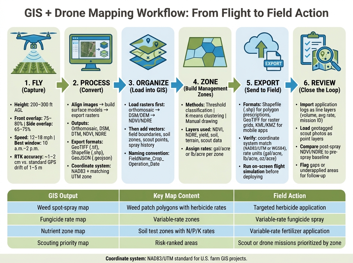
GIS + Drone Mapping Workflow: From Flight to Field Action
Step 1: Capture and process drone imagery for GIS use
Plan flights for clean, accurate field coverage
Good GIS maps start before the drone leaves the ground. The flight plan does a lot of the heavy lifting.
Fly at 200–300 ft AGL with 75%–80% front overlap and 65%–75% side overlap. Keep speed around 12–18 mph to cut motion blur, which matters even more when you're collecting multispectral imagery for NDVI. A simple lawn-mower pattern that follows the field boundary makes clipping easier later. It also helps to extend the flight grid 10–20 ft beyond the field edge so the orthomosaic fully covers headlands and no-spray zones.
Timing also plays a big part. Fly between 10:00 a.m. and 2:00 p.m. local time, when the sun is high and shadows are low. If you're running repeat flights across the season, steady lighting makes GIS comparisons much more dependable. Skip flights right after heavy rain. Standing water can throw off reflectance and vegetation index values.
RTK can make a huge difference when boundaries are tight or no-spray zones sit near waterways, neighboring properties, or residential land. Standard GPS can drift by 1–5 meters. RTK cuts that to about 1–2 cm horizontally. That kind of accuracy keeps image footprints lined up with field edges and no-spray buffers.
Turn raw images into GIS-ready map files
After the flight, move the imagery into processing software. The workflow is pretty straightforward: align images, build surface models, and export GIS-ready rasters.
The orthomosaic should be your base map. Use DSMs for canopy and terrain, DTMs for bare earth and drainage, NDVI for early vigor, and NDRE for dense canopies. For both NDVI and NDRE, you need a calibrated multispectral camera and a reflectance panel image captured before each flight.
Clean exports save time during GIS import and help avoid headaches later. Export rasters as GeoTIFF (.tif). Export vector layers such as boundaries and no-spray zones as shapefile (.shp) or GeoJSON (.geojson). Use one naming pattern across the board, like FarmName_FieldID_2026-06-15_NDVI.tif, and sort files by farm, field, and date.
Before importing, do a quick review:
- Check that the coordinate system is correct. In the U.S., NAD83 with the matching UTM zone is standard.
- Look for stitching issues along field edges.
- Make sure visible features, such as roads or field entrances, line up with your current GIS layers.
If something is off here, fix it now. A small alignment problem at this stage can turn into a prescription mistake later.
Once the files pass that check, load them into GIS and sort them by field and date.
sbb-itb-3b7eef7
Step 2: Import drone outputs and organize farm layers in GIS
Load raster and vector files into one farm map
Once the export is done, pull the drone files into your GIS project and line them up with your field records. The cleanest way to do it is to load raster layers first. Start with the orthomosaic as the base map. Then add the DSM or DEM for elevation and drainage. After that, bring in vegetation index layers like NDVI or NDRE. When those are in place, add your vector layers: field boundary polygons, scouting points, soil sampling locations, past application zones, and irrigation lines. If you are using sprayer drones for these applications, ensure the GIS layers are exported in a format compatible with the drone's controller. [7][3]
Before you load boundary and soil layers, set the project CRS to match the drone outputs. Even a small mismatch can shift features enough to put treatment zones outside the field. After import, check that every layer lines up at one known location before you start building zones. Once alignment looks right, group the layers in a way that keeps the map easy to use all season.
Use clear names, folders, and dates for repeat work
Bad naming turns a clean GIS project into chaos fast. The fix is simple: use one naming pattern and keep it the same across every field, every date, and every person on the team.
Use FieldName_Crop_Operation_Date for files. For example: North40_Corn_Scouting_09-10-2026. For layer groups, sort them by job, such as Current Imagery, Historical Imagery, Scouting, and Applications. [5][6] That way, an operator can open the right group and get to the needed layer without digging through a pile of unrelated files.
It also helps to keep a field name key, even if it’s just a basic spreadsheet. If one person says "Home Place" and another says "South Pivot", that key ties those local names back to the GIS layer IDs used in the project. [4] It sounds small, but it cuts down on mix-ups when a team works across a lot of fields.
Add labels and attributes the spray and scouting teams can use
Attributes are what turn a GIS layer from a map into a working tool. For scouting point layers, keep only the fields that help someone make a decision: crop, issue type, date observed, and a short scout note. [3][8]
For spray zone polygons, add the details the crew needs in the cab or at the shop:
- Planned rate in gal/acre
- Product name
- Application window
- Status: approved, pending, or completed
That status field can save a surprising amount of back-and-forth when several people are tracking the same field over a few days.
Step 3: Build management zones and export maps for spraying
Create management zones from imagery and field data
With the layers from Step 2 organized, the next move is to turn that field data into spray zones the crew can use in the field. The aim is simple: split the field into areas with different spray rates, or mark parts of the field as no-spray, based on what the data is telling you.
Start with NDVI or NDRE as your base layer. Then check those trouble spots against RGB imagery so you’re not making calls off one layer alone. Bring in yield, soil, terrain, and scout polygons as support. It helps to scale each layer to the same range so one layer doesn’t outweigh everything else. From there, weight the layers based on what matters most in that field, run a weighted overlay, classify the output into zones, and then clean up the boundaries by hand.
After classification, convert the raster zones into polygons. Then remove slivers or tiny fragments that equipment can’t handle cleanly. If a sprayer or drone can’t act on a shape in a clean pass, that shape probably needs to go.
Assign rates and export prescription-ready files
Each polygon needs an attribute table the controller can read. At a minimum, include:
FIELD_IDZONE_ID-
RATE_CLASS(No_Spray / Low / Medium / High) -
RATE_GPAfor liquid products in gallons per acre -
RATE_LBPAfor dry materials in pounds per acre PRODUCT_CODECOMMENTS
RATE_CLASS tells the operator what to apply in each zone. COMMENTS is where field notes go, such as "border zone" or "drainage issue."
Before exporting, check what format your equipment expects. Shapefiles (.shp, .shx, .dbf, .prj) are the most common choice for polygon-based prescriptions. They work well with spray drones like the DJI Agras series and the Talos T60X. GeoTIFF is a good fit when the device wants a raster-based rate grid. KML/KMZ can be handy for mobile apps and some drone mission planners, but attribute support can be more limited. It’s smart to load a test zone into the controller first and make sure the rate and units display the way you expect.
Choose a zone-building method that fits the job
The best method depends on how messy the field is and how much data you’ve got to work with. Some fields are clean and obvious. Others are a patchwork, and that changes the workflow.
| Method | Data Needed | Setup Effort | Best Uses | Export to Prescription |
|---|---|---|---|---|
| Threshold-based classification | NDVI/NDRE, yield, or DEM rasters | Low–moderate | Spot herbicide or fungicide zones with clear vigor differences | High - direct reclassification to polygons |
| Clustering (e.g., k-means) | Multiple rasters + multi-year data | Moderate–high | Variable fertility and nitrogen management on mixed-soil fields | High - cluster output converts cleanly to polygons |
| Manually drawn zones | Any imagery or field knowledge | Low–high depending on field size | Irregular weed patches, obstacles, irrigation patterns, and grower-known problem areas | Moderate - polygons drawn by hand, attributes added manually |
Pick the method that matches the field and the data you have on hand. Once exported, those zones are ready to use for spraying and scouting.
Step 4: Turn GIS Maps into Scouting and Spray Actions
Send Maps to the Field for spray missions and scouting routes
Once prescriptions are exported, the next move is to load them into the field device. Add the prescription package to the mission planner or mobile GIS app through USB, SD card, or cloud sync. Before import, make sure the controller uses the same coordinate system. In many U.S. farm setups, that means NAD83/UTM or WGS84 lat/long.
Check the application units too. A small mismatch here can cause big trouble in the field. Make sure rates are shown in gallons per acre, pounds per acre, or ounces per acre, depending on the job. Then compare the map against basemap imagery to see if field boundaries line up with roads, tree lines, and field edges. It also helps to run a quick on-screen flight simulation. That simple check can show whether no-spray zones and obstacles appear where they should before a single drop is applied.[10][11]
Bring Results Back into GIS After the Job
When the job is done, bring the mission data back into GIS to check coverage and rate. Import application logs and flight records as line layers that include total volume, average rate, and mission ID. When you lay those tracks over the original prescription zones, it's much easier to spot what happened in the field. You can see which areas got the planned rate and which ones did not. Any gaps or underapplied sections can then be flagged for a follow-up pass.[1][12][13]
Scout data matters just as much. Load geotagged photos and notes as point layers with the date, scout ID, issue type, and severity. If you fly follow-up imagery a few days after a spray mission, process it into a new NDVI or NDRE layer and compare it straight to the pre-spray baseline. That side-by-side view helps confirm whether the treatment worked or whether the field needs another pass.[1][12][13][2][9][14]
Conclusion: Keep the GIS-Drone Workflow Simple, Repeatable, and Field-Ready
The goal is simple: use the same workflow each time - capture, process, organize, zone, export, fly, and bring results back into GIS. When that routine stays consistent, maps stay usable, records stay clean, and the next field decision gets a lot easier.
Here’s how common GIS outputs connect to field work:
| GIS Output | Key Map Content | Field Action |
|---|---|---|
| Weed spot-spray map | Polygons of weed patches with herbicide rate attributes | Targeted herbicide application only within mapped patches |
| Fungicide rate map | Management zones with variable fungicide rates | Variable-rate fungicide spray across the full field |
| Nutrient zone map | Zones classified by soil test or crop response with N, P, K, or lime rates | Variable-rate fertilizer or lime application by zone |
| Scouting priority map | Areas ranked by risk level or previous issues | Scouts or drone missions focus first on high-priority zones |
Keep the map simple, keep the exports clean, and keep the feedback loop steady. That’s how a GIS project becomes something crews trust at the edge of the field.
FlyGuys "Integrating Drone Data into Your GIS Workflow" Webinar
FAQs
Why do my drone maps shift in GIS?
Drone maps usually shift in GIS for two main reasons: CRS mismatches and uneven spatial data between your drone imagery and the base map.
If your layers use different coordinate systems, they can drift out of place. A common example is WGS84 on one layer and a local projection on another. On screen, that small setup issue can turn into a map that doesn’t line up.
Accuracy on the drone side matters too. If you use standard GPS instead of RTK, errors can reach up to 5 feet. That’s enough to throw off measurements, boundaries, and overlays.
To cut down on shifting:
- Use the same CRS across all layers
- Use RTK for better positioning
- Add Ground Control Points (GCPs) to anchor the imagery
That combination helps your drone map line up much better inside GIS.
Do I need RTK for farm drone mapping?
Yes. RTK (Real-Time Kinematic) is the gold standard for farm drone mapping because it delivers the centimeter-level accuracy needed for variable-rate spraying and precise field boundary alignment.
With RTK-enabled drones, imagery fits cleanly into GIS software and equipment guidance systems, with horizontal accuracy that usually falls between 3 and 5 cm. For high-precision work, Drone Spray Pro offers RTK-enabled drones and accessories, including RTK dongles.
Which file format should I export for spray zones?
It depends on the drone system you use.
For DJI Agras models, export the prescription data as a Shapefile. Then place the TIF and TFW files inside a DJI folder on the microSD card.
For XAG systems, export spray zones in KML and JSON.
In every case, use WGS84 (EPSG:4326) so the GPS lines up the spray map correctly during spraying.
