How GIS Turns Drone Images into Field Maps

A drone image is just a picture until GIS ties it to the field. I’d sum it up like this: GIS links each pixel to a map location, trims the image to field edges, adds layers like obstacles and no-spray zones, and turns crop stress into scouting points or spray zones you can use.

Here’s the short version:

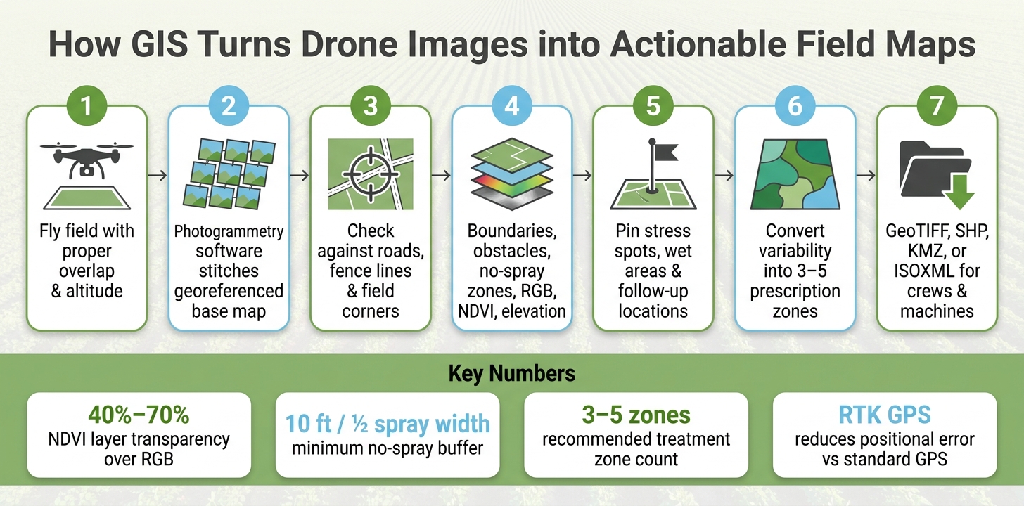
• I start with drone photos and process them into an orthomosaic
• I check map alignment against roads, corners, or fence lines
• I add field boundaries, hazards, and buffers
• I stack layers like RGB, NDVI, elevation, and notes
• I mark stress spots, wet areas, and follow-up points
• I turn those patterns into 3–5 treatment zones
• I export files like GeoTIFF, SHP, KMZ, or ISOXML for crews and machines

A few points matter most:

• Overlap affects stitch quality and map shift
• RTK can cut location error versus standard GPS
• 40%–70% transparency helps when viewing NDVI over RGB
• 10 feet or half the spray width is a common buffer around tree lines
• Wrong coordinate settings can make a field file unusable in the truck or at the edge of the field when using a DJI Agras T50 Sprayer Drone

If I had to put the whole article into one line, it’s this: GIS turns drone data into a map you can scout from, spray from, and save for later comparison.

The rest of the piece walks through that job from photo processing to field export, using plain steps a grower, scout, or spray crew can follow.

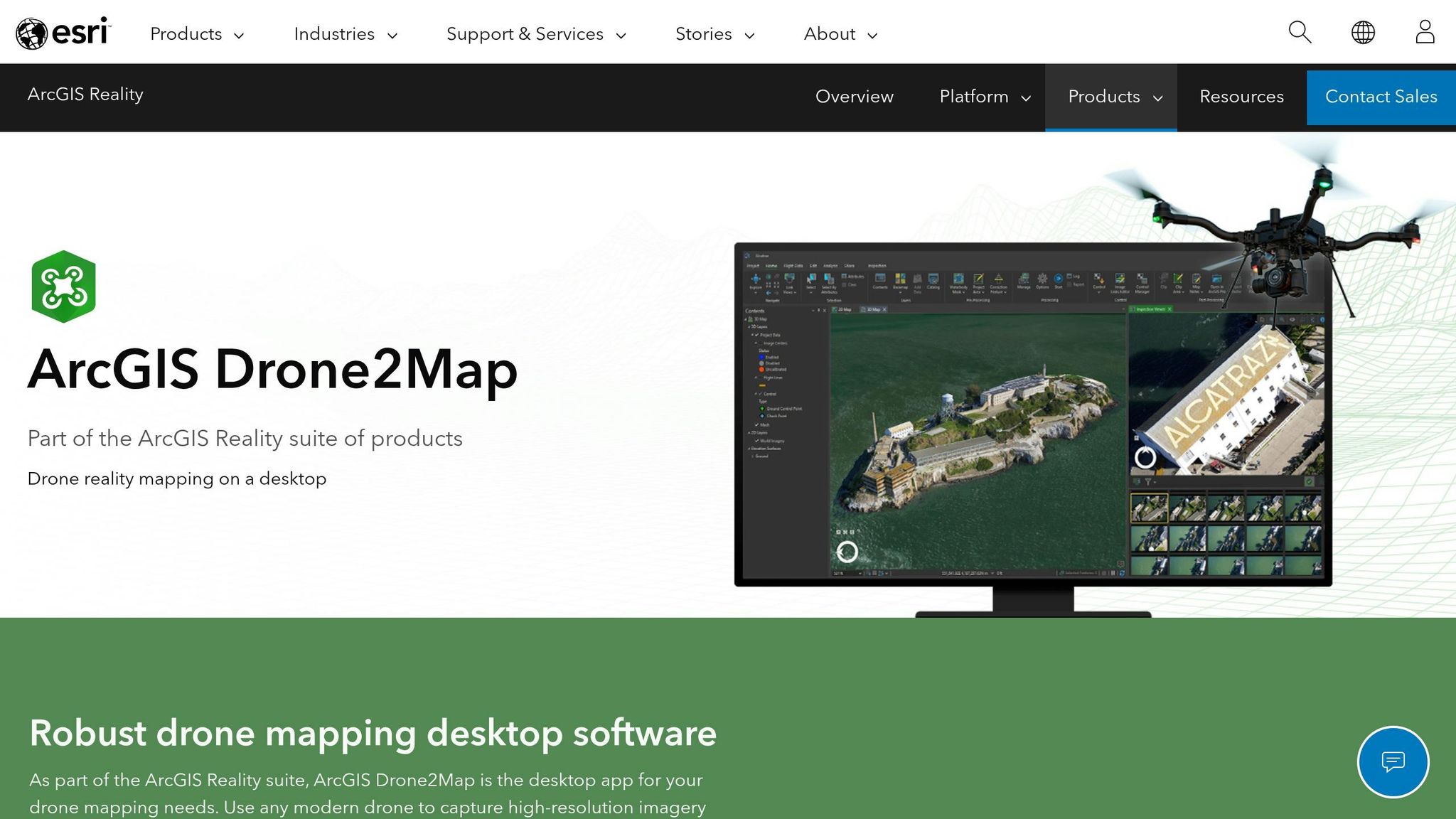
IGIS Presentation - Drone Image Processing with ArcGIS Drone2Map

sbb-itb-3b7eef7

Capture and Processing: Turning Photos Into a Georeferenced Base Map

Before GIS can do anything useful, the imagery underneath it has to be reliable. After you capture the image set, the next step is turning those photos into a map GIS can trust. If the capture is sloppy, the map will be too. And that starts with the flight itself.

Flight Settings That Affect Map Accuracy

Overlap is one of the biggest factors in capture quality. For agricultural mapping, you need enough front and side overlap so photogrammetry software can match features across photos and stitch them into a clean map. When overlap is too low, you get gaps and misalignment. That hurts boundary placement and acreage accuracy.

Altitude, speed, and camera angle matter too. Keep those settings steady across the whole flight. It also helps to keep lighting as even as possible and avoid shadows, wind, and motion blur.

If your drone supports RTK (Real-Time Kinematic) positioning, use it. RTK improves the accuracy of image locations, which helps the finished map line up more closely with field features on the ground. Without RTK, standard GPS can introduce enough positional error to push boundaries or buffer areas out of place.

From Separate Photos to Orthomosaics and Surface Models

Once the flight is finished, the raw images move into processing software. GIS and photogrammetry software turn separate photos into a georeferenced base map through photogrammetry. The software finds matching features across overlapping images and stitches them into a single, flat orthomosaic.

An orthomosaic removes tilt and terrain distortion, so each pixel gets a real-world coordinate. That makes distances, acreage, and boundaries much more dependable. The same processing run can also produce a DSM for elevation and NDVI for crop vigor. From there, GIS can use the map as a base layer for field boundaries and management zones.

Before you move into GIS analysis, check that the processed map lines up with the physical field. Import the exported boundary in KML/KMZ or shapefile (.shp) format, then compare it against fence lines, roads, or field corners. If the map is shifted here, every layer built on top of it will be shifted too.

With the base map aligned, GIS can start layering in field structure, restrictions, and scouting data.

How GIS Adds Field Structure With Boundaries and Layers

A clean orthomosaic is a starting point, but by itself, it’s just a picture. GIS adds the missing context. It turns imagery into a working map with polygons, lines, points, and attribute tables so a farm team can answer three basic questions fast: Where is this? Which part of the field is it? What needs to happen here?

Draw or Import Field Boundaries, Obstacles, and No-Spray Areas

The first layer to add is the field boundary. You can import one that already exists or trace a new one directly over the orthomosaic. Follow visible edges like fence lines, road margins, or irrigation ditches. Then add details such as Field ID, crop, and acreage so crews using a DJI Agras T40 can spot the right field without any guesswork.

Once the boundary is in place, clip the orthomosaic to that polygon. That way, operators see only the field they’re working on, not all the extra area around it.

From there, add separate layers for obstacles and no-spray areas. Power poles and transmission lines usually work best as points and polylines. Waterways, homesteads, and other sensitive spots are often mapped as polygons with buffer zones. Around tree lines and similar features, use a no-spray buffer of at least 10 feet, or half the spray width.^[1] Each layer can also store fields like Buffer_ft, Hazard_Type, and Last_Checked_Date, which gives pilots useful context before a flight. This data is especially critical when operating high-capacity systems like the DJI Agras T50 in complex environments.

Use Layer Stacking to Compare Crop Conditions and Field Features

Once the field is outlined, layers shift the map from simple reference to day-to-day decision support.

The main step here is stacking multiple layers over the base imagery. A common setup puts the orthomosaic at the bottom, then adds a vegetation index layer like NDVI at partial transparency - usually around 40% to 70% - so you can see both the vigor pattern and the crop rows underneath. Boundaries, no-spray zones, and obstacle markers stay on top so they don’t get lost in the image. It also helps to save preset views like Scouting and Spray so crews can switch between them fast.

A practical setup often looks like this:

• RGB for visual checks
• NDVI/NDRE for vigor
• Boundaries for treated acres
• Obstacles for safe paths
• No-spray zones for compliance
• Notes for follow-up scouting

With those layers in place, GIS starts to turn field variability into clear scouting and spray zones.

Build Scouting Zones and Spray Prescription Areas

With field boundaries, obstacles, and stacked layers already in place, the next step is turning what you see on the map into zones your crew can use in the field. This is the point where GIS stops being just a reference and starts driving action.

Mark Stress Areas, Hotspots, and Priority Scouting Locations

Start by scanning NDVI and NDRE for patterns that line up with RGB imagery and field features. Look for low-vigor bands, bare spots, dark or shiny areas that may point to standing water, and linear stress tied to drainage paths or compaction lines.

When you find something that needs a closer look, drop a pin for one exact spot, draw a polygon around a bigger stress area, or trace a line along an erosion rill or runoff path. For each pin, add the issue, date, growth stage, and source layer. Then assign one status label: stress, water, or verified.

That simple setup helps scouts work fast. They can open the pins in the field, check the cause, and update the note on the spot.

Once the field is marked up, GIS turns those notes into management zones.

Convert Variability Into Treatment Zones

After scouting confirms what’s happening, the same map can be used as a prescription map. Set up 3–5 vigor classes, or let the software group the raster into natural zones. GIS then converts those classes into polygons and tags each one with a class ID plus a rate code or an on/off command.

From there, the map can guide:

• Spot treatment
• Edge treatment
• Variable-rate application

Weed distribution maps derived from UAV imagery can also be converted into variable spray prescription maps, supporting variable-rate spraying and improving pesticide efficiency.^[2]

These zones are then exported for field use.

Export the Map for Field Use and Next Steps

Export Formats That Make Drone Maps Usable

Once GIS turns field variability into zones, the next step is simple: get those layers into the right hands. Exporting is what moves a map from the office to the scout, spray crew, or machine console that will use it.

Here are the main export types and where they fit:

Format	Best For	Notes
GeoTIFF	Orthomosaics, NDVI layers, elevation models, office review	Best for raster review and measurement
Shapefile	Field boundaries, no-spray zones, prescription polygons	Widely supported by farm software, GIS tools, and machine terminals
KML/KMZ	Scouting crews, tablet viewing	Easy to open in mobile apps; not ideal for machine execution
ISOXML	Variable-rate sprayers, tractor consoles	Carries zone boundaries and rate instructions for compatible terminals

Use the format that your sprayer, tablet, or GIS stack can read. That sounds obvious, but it saves a lot of frustration in the field.

Before you export, make sure the file matches the device that will open it. Check that the coordinate system lines up with what the target device expects, the resolution fits the device’s storage and processing limits, and the attribute fields in prescription files include valid rate values.

For offline field work, load a KMZ overlay and the needed vector layers onto tablets or controllers before heading out. If you skip that step, a clean map can turn into a headache fast.

With the right files ready to go, crews can scout, spray, and document the field without having to rebuild or fix the map first.

Conclusion: From Images to Actionable Field Maps

The workflow follows a clear path: raw drone photos → georeferenced orthomosaic → GIS-structured field map → scouting zones and prescription areas → exported files for crews and machines. Export is the last step that puts mapped zones in front of the people doing the job.

Drone Spray Pro supports ag spray drone workflows with training, FAA licensing help, and accessories like batteries, chargers, and RTK dongles.

FAQs

Why isn’t a drone photo enough by itself?

A raw aerial photo isn't enough for farm decisions because it doesn't have the spatial structure or context you need. On its own, it's just a flat image, not georeferenced data.

GIS turns that image into a map you can use. It lines the photo up with GPS coordinates and adds layers like field boundaries, notes, and zone data. Once that happens, it's much easier to spot coverage gaps, check crop health, and direct scouting and spray decisions.

How accurate does a drone map need to be for spray work?

For spray work, drone maps need tight positional accuracy so treatments line up with exact crop rows or stress zones. Standard drone GPS usually misses that mark. With horizontal errors of 10 to 16 feet, it’s often too far off for precise application.

That’s where RTK or GCPs come in. They’re needed for centimeter-level precision, which makes a big difference in the field. Better map accuracy can cut spray overlap by up to 23% and helps make sure inputs go only where they’re needed.

Which export file should I use for scouting or spraying?

For scouting and spraying, Shapefile (.shp) is the best export format. It's the standard for prescription zones, and it works with most spray drone controllers, tractor terminals, and farm management software.

For variable-rate application, include these fields:

• rate
• rate integer
• unit
• zone ID

If you only need simple boundaries or flight planning, KML or KMZ can work well too. Use WGS84 to keep GPS alignment accurate.

Related Blog Posts

• How Topographic Mapping Improves Spray Drone Accuracy
• How to Use Drone Data for Yield Optimization
• How AI Detects Field Variability with Drones
• How to Combine Satellite and Drone Data for Field Zoning