
Call or Text: +1 (208) 425-2990
Email: Sales@DroneSprayPro.com

CNN vs ViT for Aerial Pest Classification
I’d start with a pretrained CNN when labels or hardware are limited, and test a ViT when canopy-wide patterns matter. A hybrid is worth testing only if combining local detail with context improves results enough to justify its added cost.
First, check what your aerial images can show: pest species, damage symptoms, or infestation severity. A model can’t identify an insect that occupies too few pixels. Resolution also affects compute: doubling image width and height at the same ViT patch size creates 4× as many tokens and about 16× as many full-attention pairs.
Quick Comparison
| Criterion | CNN | ViT | CNN–Transformer hybrid |
|---|---|---|---|
| Main strength | Local textures and damage cues | Relationships across image regions | Local detail plus spatial context |
| Limited labels | Pretrained models are a useful starting point | Pretraining quality matters | Test against simpler models |
| Image size | Downsampling may remove small cues | Resolution and patch size affect detail and memory | Depends on the design |
| Compute and training | Compact models often fit tight limits | Full attention can demand more memory | Added blocks can increase training and inference costs |
| Deployment cost | Benchmark on different drone models | Check latency and memory at the chosen resolution | Require a measured gain before accepting extra cost |
I’d compare all candidates using the same sensor inputs, preprocessing, and fields held out from training. Measure macro-F1, per-class recall, training time, memory, device latency, and total cost in U.S. dollars - including labeling and human review. Then check performance on new fields and seasons.
<u>A class score is not a treatment map. Once you have validated your data, you can deploy results using professional sprayer drones.</u> Before spraying, I’d require location checks, field scouting, and review of applicable FAA rules, state pesticide requirements, and label directions.
ViT vs CNN: A Comparative Experiment
sbb-itb-3b7eef7
CNN vs ViT: How They Work and Where They Fall Short
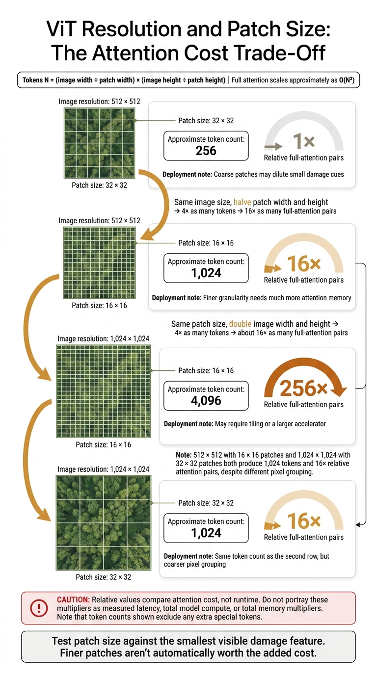
ViT Resolution and Patch Size: The Attention Cost Trade-Off
CNNs favor local detail; ViTs favor broader image context. Pretraining, resolution, and hardware help determine which model fits your task. Start by matching each model’s strengths to the smallest pest cue visible in your drone images.
| Aspect | CNNs | ViTs with full self-attention |
|---|---|---|
| Local features | Strong built-in bias toward nearby edges, textures, color patterns, and shapes | Learn features from patch representations; large patches can dilute tiny cues |
| Spatial context | Build larger receptive fields through depth and pooling | Directly relate distant image patches |
| Transfer learning | Established pretrained CNN families are commonly used for limited-label tasks | Strong pretraining matters especially when labels are limited[6] |
| Resource needs | Compact variants often fit constrained hardware | Full-attention costs grow sharply with resolution and token count |
| Main limits | Downsampling can remove tiny cues; occlusion and background shortcuts remain | Patch size, pretraining quality, and attention memory constrain performance |
CNNs for Local Pest and Damage Features
Use CNNs when visible damage depends on local detail. Convolutional filters learn edges and color transitions, then combine them into textures, discoloration, curled foliage, pest bodies, and damaged canopy patterns - provided those cues are visible.
With limited labels, start with a pretrained model: replace its head, train the new head with the backbone frozen, then unfreeze deeper layers at a low learning rate. Changes in scale, occlusion, and hidden foliage can still cause recognition failures. Include hard negatives such as healthy canopy, soil, and shadows to discourage the model from relying on background shortcuts.
| CNN family | Parameter efficiency and training needs | Field inference |
|---|---|---|
| ResNet | Residual connections make deeper networks easier to optimize; ResNet-18 or ResNet-50 commonly suit transfer learning | Established tooling; compare small and larger variants on the intended device |
| EfficientNet | Uses compound scaling to balance depth, width, and resolution; input-size choices matter | Useful for balancing accuracy and compute; higher-resolution variants increase latency |
| MobileNet | Designed for low parameter count and low multiply-accumulate cost; supports pretrained fine-tuning | A strong candidate for constrained hardware, though smaller variants may miss subtle damage |
| ConvNeXt | Updates CNN design while retaining convolutional inductive biases; gains from large-scale pretraining | Better suited to capable accelerators than very limited onboard computers |
ViTs for Context Across Image Regions
Use ViTs when the label depends on canopy-wide patterns rather than local texture alone. A ViT projects image patches into tokens, adds positional information, and uses self-attention to relate them.[5] This lets it compare a damaged patch with surrounding rows and canopy context. But if resolution is too low, patching can erase tiny cues.
| Image resolution | Patch size | Approximate token count | Relative full-attention pairs | Deployment note |
|---|---|---|---|---|
| 512 × 512 | 32 × 32 | 256 | 1× | Coarse patches may dilute small damage cues |
| 512 × 512 | 16 × 16 | 1,024 | 16× | Finer granularity needs much more attention memory |
| 1,024 × 1,024 | 16 × 16 | 4,096 | 256× | May require tiling or a larger accelerator |
| 1,024 × 1,024 | 32 × 32 | 1,024 | 16× | Same token count as the second row, but coarser pixel grouping |
Relative values compare attention cost, not runtime.
Full attention scales approximately as O(N²) with token count. Test patch size against the smallest visible damage feature. Finer patches aren't automatically worth the added cost.
Hybrid Models for Local Features and Spatial Context
Use a hybrid only when CNN detail and ViT context both matter for the same pest label. CNN–Transformer hybrids pass locally extracted features into blocks that learn spatial relationships.[7][8] Compare each hybrid with its CNN baseline to check whether added context improves pest recall enough to justify extra memory, latency, and tuning.
| Model type | Features used | Implementation complexity | Hardware fit |
|---|---|---|---|
| CNN | Local patterns and progressively broader features | Low to moderate | Compact variants suit edge devices |
| ViT | Patch features linked by attention | Moderate to high | Full attention favors capable GPUs; compact or windowed variants reduce demands |
| Hybrid | Convolutional features plus learned spatial relationships | Often higher; additional components need tuning | Depends on design; benchmark compact hybrids rather than assuming they suit edge devices |
Compare Image Size, Data Needs, Compute, and Training Time
Keep the comparison consistent: use the same classes, field-separated splits, preprocessing, augmentation, balancing, and tuning budget. Keep all tiles from the same flight or field in one split.[11][13] With evaluation held constant, test whether resolution, label count, and compute change which model performs best.
Image Resolution and Patch Size
Report both original and model input dimensions in pixels. Include flight altitude in feet with metric equivalents, the camera/sensor model, and ground sampling distance (GSD) in inches per pixel with centimeters-per-pixel equivalents.
Also record the target’s size in pixels. Insects, feeding patterns, and canopy symptoms require different levels of detail. Document tile dimensions, overlap percentage, padding, prediction-merging method, tiles per acre, and total processing time.
| Input choice | Benefit | Cost or check |
|---|---|---|
| Resize the full image to 224 × 224 px | Fewer pixels to process | Check whether small symptoms remain visible |
| Tile at native resolution | Keeps local detail | More predictions; less surrounding context |
| Overlap tiles | Helps preserve edge objects | Merge duplicate outputs; keep tiles from the same field in one split |
For square patches, token count grows with image area. Full-attention cost grows with the square of the token count.
At 16 × 16 patches, 512 × 512 images produce 1,024 tokens versus 196 for 224 × 224. Attention interactions increase by about 27.3×, but total runtime also depends on width, depth, and implementation.[14][15][16]
Next, check whether each model maintains its performance across fields and seasons.
Labeled Data and Performance Across Fields
No label count guarantees reliability. Pretrained ViTs can learn long-range relationships, but small datasets or shifts in the data often call for stronger pretraining, regularization, and augmentation.[9][10]
Include varied crops, relevant cultivars, growth stages, pest severity levels, locations, management practices, sensor conditions, flight heights, lighting, and backgrounds.
Split before tiling. Keep each field, its flights, adjacent frames, and repeated plot observations together. Hold out entire fields for testing - and preferably at least one season, location, or flight campaign. Report counts for fields, flights, dates, images, tiles, and examples per class separately.[12]
| Approach | Limited-data use | Pretraining and labeling checks |
|---|---|---|
| Pretrained CNN | Useful baseline for local damage cues | Verify performance on field-separated splits |
| Pretrained ViT | More sensitive to small datasets or domain shifts | Test checkpoint suitability; natural-image pretraining is not automatically best |
| CNN–Transformer hybrid | Worth testing when both detail and context matter | Use the same tuning budget |
Then compare the hardware demands each model brings to field deployment.
Hardware Costs and Training Time
To make the experiment reproducible, record hardware, software, precision mode, batch size, epochs, optimizer, learning rate, scheduler, weight decay, warm-up, checkpoint rule, and early-stopping patience.
| Model | Input dimensions | Patch size | Parameters | Model file size | FLOPs | Peak GPU memory | Training time | Inference latency |
|---|---|---|---|---|---|---|---|---|
| CNN baseline | NR | N/A | NR | NR | NR | NR | NR | NR |
| ViT baseline | NR | NR | NR | NR | NR | NR | NR | NR |
| CNN–Transformer hybrid | NR | NR | NR | NR | NR | NR | NR | NR |
NR = not reported or not measured. State whether FLOPs means floating-point operations or multiply-accumulate operations, and identify the profiling tool and version. Do not infer missing values from parameter count or published results.
Measure training time from the first batch to the selected checkpoint, and report tuning time separately. On the intended device, document runtime, export format, FP32/FP16/INT8 settings, batch size, warm-up and timed-run counts, and median and 95th-percentile latency.
Record peak memory and latency at realistic tile counts. State whether measurements include transfer, preprocessing, and postprocessing.
After export or quantization, reevaluate accuracy, macro-F1, per-class recall, calibration, file size, peak memory, and target-device latency on the same untouched field-separated test set.
Estimate training and inference costs separately in U.S. dollars, using documented rates or hardware ownership costs. Document the date of those assumptions; leave estimates NR if no rate is available. Speed depends on the configuration - not the architecture name alone.
Test Models and Plan Farm Deployment
Test on Separate Fields and Seasons
Once a model clears the benchmark, test it on fields and seasons it hasn’t seen. Validate the ResNet/EfficientNet baseline, pretrained ViT, and optional hybrid on held-out fields. Choose geographically separate fields and, when possible, a later season to see which model transfers best.
Report macro-F1, balanced accuracy, per-class recall, confusion matrices, and calibration. Count false negatives separately, paying close attention to severe infestations labeled healthy. Break down results by field, season, and pest severity, and set acceptance thresholds before reviewing results.
On the intended hardware, measure model-only latency separately from preprocessing, transfer, georeferencing, and total workflow time. If the model passes field-held-out testing, check whether it meets the farm’s turnaround and hardware limits.
Match the Model to Farm Limits
Test each candidate using the same field-held-out protocol. Post-flight processing supports heavier compute, but uploads delay decisions. On-board inference must stay within power, heat, memory, and offline limits.
| Farm condition | Model candidate | Required validation | Deployment trade-off |
|---|---|---|---|
| Limited labels or strict turnaround limits | Efficient CNN, such as ResNet or EfficientNet | Compare against a pretrained ViT on held-out fields; report recall on rare pests | A practical starting point for local use; may miss broader spatial context |
| Spatial patterns matter and suitable pretrained weights are available | Pretrained ViT | Test patch-size sensitivity, new-season performance, calibration, and memory use | Broader context may help; larger inputs can increase compute |
| Small symptoms and surrounding canopy both matter | CNN–Transformer hybrid | Run ablations; compare accuracy, latency, and failure cases | Added complexity must produce a measurable gain |
| Weak connectivity or near-aircraft feedback is required | Efficient CNN or compressed hybrid | Benchmark offline operation, thermal stability, energy use, and compressed-model accuracy | Less data transfer, but tighter hardware limits |
| Service business covers multiple crops or farms | Compare all candidates by operating condition | Use farm-held-out tests, test sensor differences, and monitor drift | More validation and maintenance; don’t assume one model will work reliably everywhere |
If the model becomes part of a spray workflow, verify its output before treatment.
Turn Predictions Into Verified Treatment Maps
A class score is not a spray map. Locate damage with georeferenced tiles or a separate detection/segmentation step. Check GPS or RTK alignment, camera timing, coordinate-system alignment, and spatial uncertainty against ground observations.
Have an agronomist or trained scout inspect uncertain areas and sample both positive and negative predictions. Block treatment when pest identity, image quality, or location is uncertain. Retain images, model versions, coordinates, and review decisions.
Before spraying, verify applicable FAA requirements, Part 107 and Part 137 obligations, state pesticide credentials, and label directions permitting aerial application. Follow label rates, buffers, weather limits, and safety requirements.
Conclusion: Choose Field-Tested Performance Within Budget
After field-held-out testing, start with a pretrained CNN if labels are limited or hardware limits are tight. Choose a pretrained ViT when canopy-scale context drives the label. Use a hybrid only if it outperforms the simpler model on the same test set.[4][20][19]
Compare total cost, not just training cost. Rank models by field-held-out macro-F1, latency on the target hardware, and costs for labeling, tuning, retraining, and human review. Keep those trade-offs within the farm’s workflow limits.[17] Higher-resolution inputs are worth the added cost only if they preserve pest cues while staying within memory and inference limits.
Retest when flight height, camera settings, crop, or season changes.[18][21]
FAQs
How can I tell pest damage from drought stress?
Use thermal and multispectral data together. Thermal maps show hot spots caused by stomatal closure, but they can’t tell you what caused it.
The pattern offers clues. Drought stress typically follows irrigation layouts, pivot zones, or soil variations. Pest damage often shows up as localized, irregular hot spots that don’t align with terrain or irrigation.
Check NDRE within each hot spot: low NDRE makes pest or disease pressure more likely, while normal NDRE points toward abiotic factors such as drought.
How should I handle rare pests in training data?
Balance the training data for healthy and infested plants so models don’t miss rare outbreaks. One approach pairs the Synthetic Minority Over-sampling Technique (SMOTE) with Long Short-Term Memory (LSTM) networks to track and detect rare events across plant growth stages.
Tailor your AI software and training data to your crops and local conditions. Always check flagged areas in the field to confirm that pests are present.
When should I retrain my pest classification model?
Retrain your pest classification model when its training data no longer matches your farm’s conditions or its performance drops as conditions change [1]. Models can struggle with the shift from lab settings to fields. Use data that reflects your crops and local pests [1].
Use performance data from previous seasons to improve detection accuracy and treatment efficiency [2]. Regularly add new, ground-truthed data as field conditions change [3].
